Loki2 Morphological Pseudotime Inference - Colorectal Cancer Samples

This notebook demonstrates how to infer morphological pseudotime across multiple colorectal cancer (CRC) samples using Loki2 cell morphology embeddings.

Data Requirements

The example data is stored in the directory ../data/morph_psdtime, which can be donwloaded from Google Drive.

You will need:

• Loki2 cell inference results

• Loki2 cell embeddings for multiple CRC samples

• Whole slide images for visualization

import os 
import numpy as np
import pandas as pd
import scanpy as sc
import matplotlib.pyplot as plt
import matplotlib as mpl
import openslide
import plotly.express as px
import plotly.graph_objects as go
import plotly.io as pio
import palantir
from skimage.transform import rotate
pio.renderers.default = "notebook" 

import loki2.preprocess
import loki2.psdtime
import loki2.plot

Load Data

Load cell embeddings and spatial coordinates from multiple CRC samples. This section filters cells based on cell type annotations and selects a specific region of interest using a bounding box. The embeddings capture morphological features that will be used for pseudotime inference.

name = "CRC"
output_dir = f"../outputs/morph_psdtime/output/Results_{name}"
os.makedirs(output_dir, exist_ok=True)

sc.set_figure_params(dpi=200)
mpl.rcParams["axes.grid"] = False

names = ["CRC_sample3", "CRC_sample2", "CRC_sample1"]
tumor_index = {}

for name in names:
    print(name, end=', ')
    json_file = f"../data/morph_psdtime/{name}_cells.json"
    tumor_index[name] = loki2.psdtime.load_tumor(json_file, tumor_typeids=['1'])

CRC_sample3, (202206, 5)
CRC_sample2, (321549, 5)
CRC_sample1, (275640, 5)

embs_tumor = {}
locations = {}

bbox = {
    'CRC_sample3': [0, 50000, 0, 50000],
    'CRC_sample2': [0, 50000, 0, 50000],
    'CRC_sample1': [0, 50000, 0, 50000]
}

for name in names:
    input_path = f"../data/morph_psdtime/{name}_cells.pt"
    features = loki2.preprocess.load_and_print_tensor(input_path)
    embs = features.x
    embs = embs[tumor_index[name]]
    #embs = F.normalize(embs, p=2.0, dim=1)
    locs = features.positions[tumor_index[name]]
    mask = loki2.psdtime.in_bbox(locs, bbox[name])

    embs_tumor[name] = embs[mask]
    locations[name] = locs[mask]

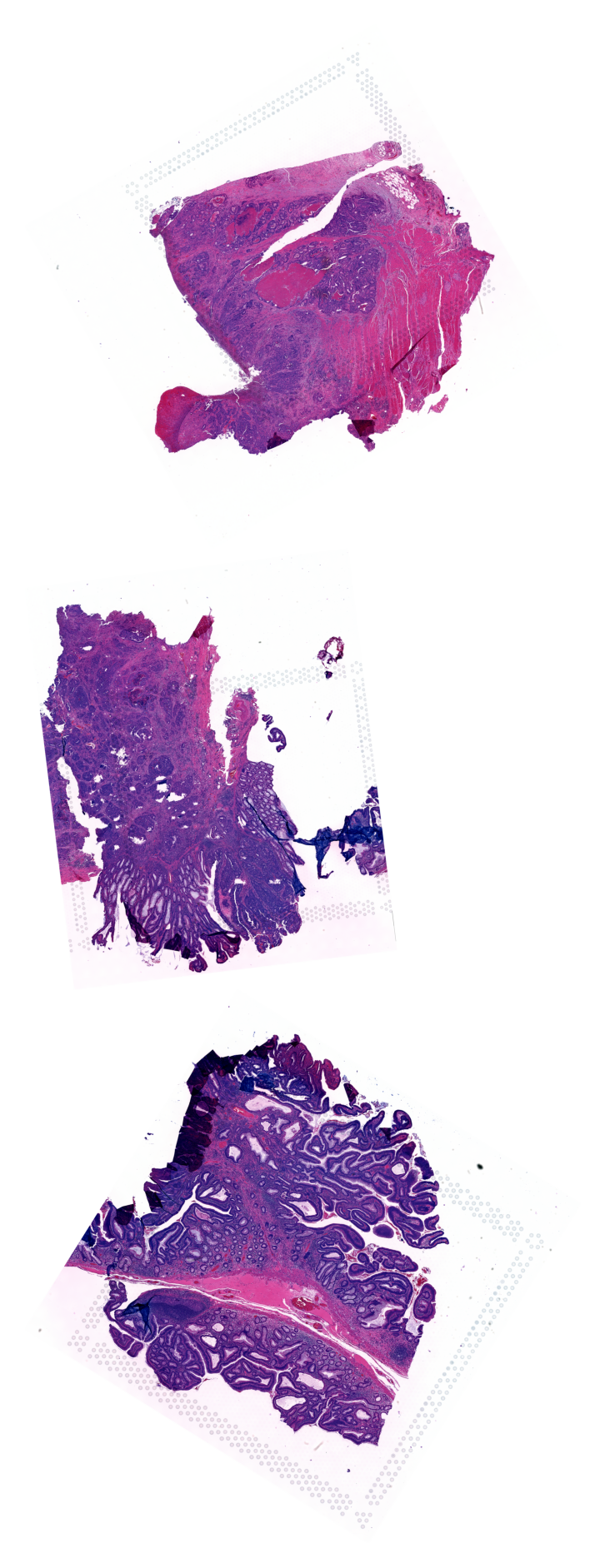
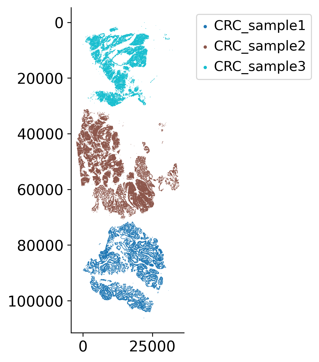
Assemble the Three Samples on One Slide for Visualization

Rotate and align multiple tissue samples spatially to create a combined visualization. This spatial alignment allows for direct comparison of samples and helps understand how different tumor grades or regions relate to each other morphologically.

image_paths = {
    "CRC_sample3": "../data/morph_psdtime/CRC_sample3.tif",
    "CRC_sample2": "../data/morph_psdtime/CRC_sample2.tif",
    "CRC_sample1": "../data/morph_psdtime/CRC_sample1.tif",
}

# Rotate the samples to align with the orientations present in the Cell paper
angles_deg = {
    'CRC_sample3': 330, 
    'CRC_sample2': 83, 
    'CRC_sample1': 122
}

max_side = 4000  # longest side of thumbnail
rot_imgs = []

for name in names:
    slide = openslide.OpenSlide(image_paths[name])
    full_w, full_h = slide.dimensions

    scale = max_side / max(full_w, full_h)
    thumb_size = (int(full_w * scale), int(full_h * scale))
    img = np.array(slide.get_thumbnail(thumb_size))  # uint8 RGB

    angle = angles_deg[name]

    # convert to float [0,1] for rotate, then back to uint8
    img_f = img.astype(np.float32) / 255.0
    img_rot = rotate(
        img_f,
        angle=360-angle,
        resize=True,           # allow expansion so no cropping
        preserve_range=False,  # output still in [0,1]
        mode="constant",
        cval=1.0,              # white background
    )
    img_rot = (img_rot * 255).astype(np.uint8)

    rot_imgs.append(img_rot)

# determine final canvas size
widths  = [im.shape[1] for im in rot_imgs]
heights = [im.shape[0] for im in rot_imgs]

max_w = max(widths)
total_h = sum(heights)

# create white canvas
canvas = np.ones((total_h, max_w, 3), dtype=np.uint8) * 255

# paste images vertically
y_offset = 0
for im in rot_imgs:
    h, w, _ = im.shape
    canvas[y_offset:y_offset + h, 0:w, :] = im
    y_offset += h

plt.figure(figsize=(4, 8), dpi=150)
plt.imshow(canvas)
plt.axis("off")
plt.show()

all_pos = loki2.psdtime.assemble_spatial(
    [locations[name] for name in names], 
    [angles_deg[name] for name in names],
)
all_pos = np.concatenate(all_pos)
samples = []
for name in names:
    samples += [name] * len(locations[name])
loki2.plot.scatter_plot(all_pos, samples, s=0.1, invert_y=True, lw=0, ec=None, palette='tab10', 
             # save_path=f"{output_dir}/sample_layout.jpg"
            )
embs = np.concatenate([embs_tumor[name] for name in names])

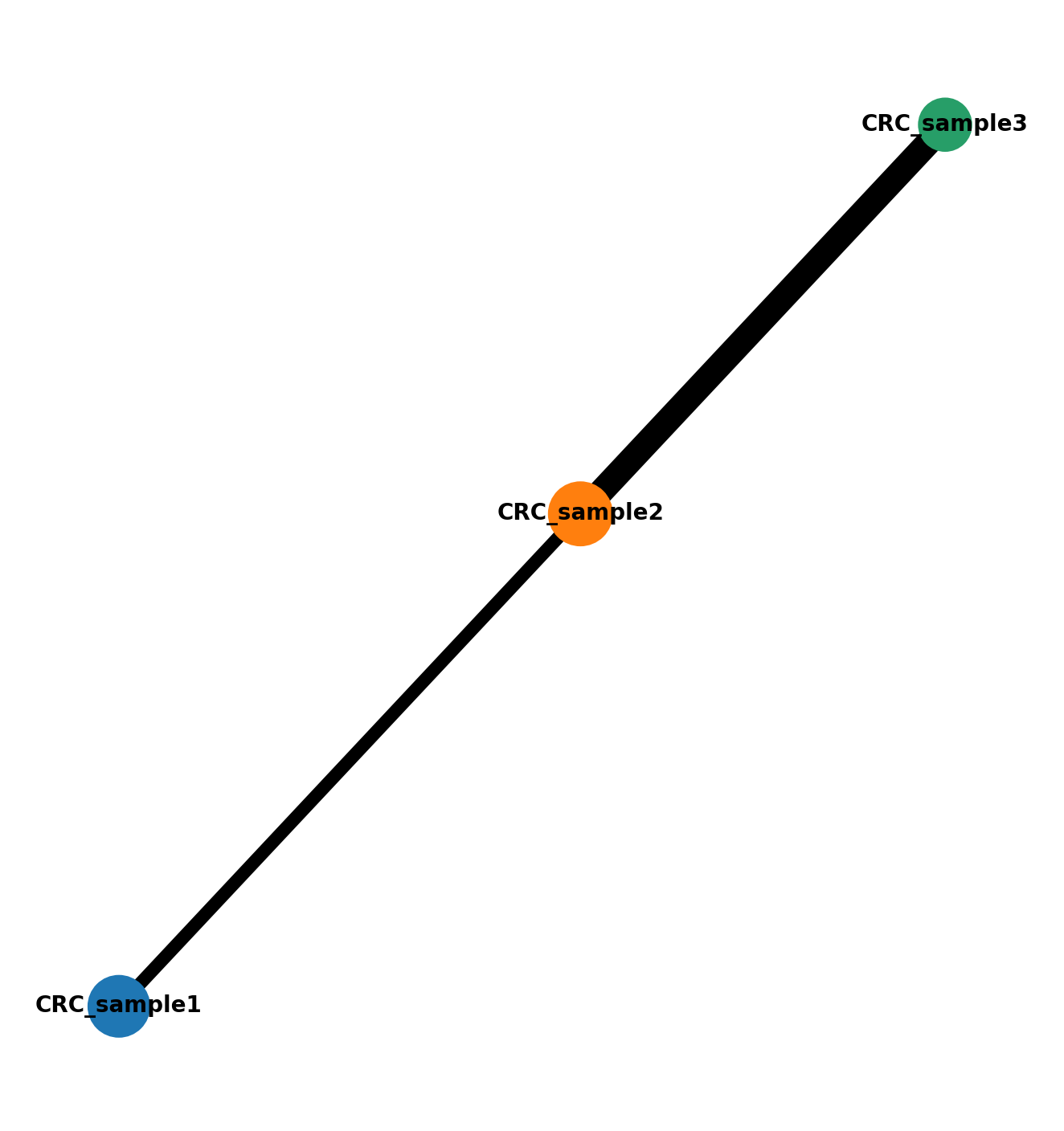
Check the Topology and Gradient in Image Embeddings Among Samples

Analyze the connectivity structure and gradients in the cell state manifold across multiple samples. This section uses PAGA (Partition-based Graph Abstraction) to understand sample connectivity and resolve coarse-grained connectivity structures of complex manifolds. The analysis helps identify how different samples and tumor grades relate to each other in the embedding space.

ad = sc.AnnData(embs)
ad.obsm['spatial'] = all_pos
ad.obsm['spatial_ori'] = np.concatenate([locations[name] for name in names], axis=0)

ad.obs['imagerow'] = ad.obsm['spatial'][:, 1]
ad.obs['imagecol'] = ad.obsm['spatial'][:, 0]
ad.obs['sample_name'] = samples

sc.pp.neighbors(ad, n_neighbors=100)

Here we run PAGA to resolve a coarse-grained connectivity structures of complex manifolds consisting of three samples and different grades

sc.tl.paga(ad, groups='sample_name')

sc.pl.paga(ad, fontsize=5, frameon=False)

sc.tl.umap(ad, init_pos='paga')

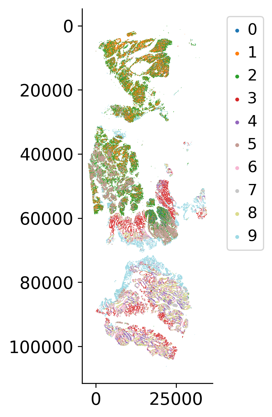
Prepare Data and Perform Clustering

Create an AnnData object from the embeddings and compute neighborhood graphs, perform Louvain clustering, and apply dimensionality reduction (UMAP). These analyses help identify distinct cell populations and capture the underlying structure of the cell state manifold, which is essential for pseudotime inference.

sc.tl.louvain(ad, resolution=1)

loki2.plot.scatter_plot(
    ad.obsm['spatial'], 
    ad.obs['louvain'],
    s=0.1, invert_y=True, lw=0, ec=None, palette='tab20',
    )

mask = ((ad.obs['sample_name'] == 'CRC_sample3') & (ad.obs['louvain'].isin(['1','2']))) | \
       ((ad.obs['sample_name'] == 'CRC_sample2') & (ad.obs['louvain'].isin(['1','2', '3', '5']))) | \
       ((ad.obs['sample_name'] == 'CRC_sample1') & (ad.obs['louvain'].isin(['3','4','8'])))

ad_sel = ad[mask].copy()

ad_sel

AnnData object with n_obs × n_vars = 186308 × 1280
    obs: 'imagerow', 'imagecol', 'sample_name', 'louvain'
    uns: 'pca', 'neighbors', 'paga', 'sample_name_sizes', 'sample_name_colors', 'umap', 'louvain'
    obsm: 'spatial', 'spatial_ori', 'X_pca', 'X_umap'
    varm: 'PCs'
    obsp: 'distances', 'connectivities'

Select Starting Cell for Pseudotime

Plot the UMAP (hover) for easier selection of an early cell. The algorithm will find a start cell near the selected cell. This interactive visualization helps identify the starting point for pseudotime inference, which represents an early developmental or progression state.

sample_name = ad_sel.obs['sample_name'].astype('string').fillna('')

df = pd.DataFrame({
    "x": ad_sel.obsm['X_umap'][:, 0],
    "y": ad_sel.obsm['X_umap'][:, 1],
    "cluster": ad_sel.obs['louvain'],
    "sample_name": sample_name,
    "sx": ad_sel.obsm['spatial'][:, 0],
    "sy": ad_sel.obsm['spatial'][:, 1],
    "cell_id": ad_sel.obs_names,
})

fig = px.scatter(
    df,
    x="x", y="y",
    color="cluster",
    color_discrete_sequence=px.colors.qualitative.T10,
    hover_data={
        "sample_name": True,
        "cluster": ":d",
        "x": ":.2f",
        "y": ":.2f",
        "sx": ":.1f",
        "sy": ":.1f",
        "cell_id": ":6d"
    },
)

fig.update_traces(marker=dict(size=1), selector=dict(mode="markers"))

legend_marker_size = 10
legend_traces = []
for trace in fig.data:
    trace.legendgroup = trace.name
    trace.showlegend = False
    legend_traces.append(
        go.Scatter(
            x=[None],
            y=[None],
            mode="markers",
            marker=dict(
                color=trace.marker.color,
                symbol=trace.marker.symbol or "circle",
                size=legend_marker_size,
            ),
            name=trace.name,
            legendgroup=trace.legendgroup,
            hoverinfo="skip",
        )
    )

fig.add_traces(legend_traces)
fig.update_layout(
    xaxis_title="UMAP-1",
    yaxis_title="UMAP-2",
    dragmode="pan"
)

fig.update_layout(width=600, height=600)
fig.show()

sc.pp.neighbors(ad_sel, use_rep='X_umap')

Infer Pseudotime

Apply Palantir algorithm to infer pseudotime from the morphological embeddings. The algorithm uses the starting cell to define the beginning of the trajectory and computes pseudotime values for all cells based on their positions in the embedding space.

start_cell = '229796'
loki2.psdtime.infer_pseudotime_palantir(ad_sel, start_cell, output_dir, f'COAD-{start_cell}', n_components=15, knn=100, num_waypoints=2000)

Kept components: 13 of 13
Sampling and flocking waypoints...
Time for determining waypoints: 0.5021961251894633 minutes
Determining pseudotime...
Shortest path distances using 100-nearest neighbor graph...
Time for shortest paths: 41.13739737669627 minutes
Iteratively refining the pseudotime...
Correlation at iteration 1: 1.0000
Entropy and branch probabilities...
Markov chain construction...
Identification of terminal states...
Computing fundamental matrix and absorption probabilities...
Project results to all cells...

Visualize Pseudotime

Visualize the inferred pseudotime values on both spatial coordinates and UMAP embedding space. The spatial visualization shows how pseudotime progresses within the tissue, revealing regions at different stages of development or progression. The UMAP visualization shows pseudotime progression in the reduced embedding space, highlighting the trajectory structure.

loki2.plot.scatter_plot(
    ad_sel.obsm['spatial'], 
    ad_sel.obs['palantir_pseudotime'], 
    s=0.1, invert_y=True, lw=0, ec=None, palette='viridis', equal_aspect=True,
    # save_dpi=200,
    # save_path=f"{output_dir}/pseudotime_on_spatial.jpg"
    )

loki2.plot.scatter_plot(
    ad_sel.obsm['X_umap'][:, :2], 
    ad_sel.obs['palantir_pseudotime'],
    s=0.1, invert_y=False, lw=0, ec=None, palette='viridis',
    # save_dpi=200,
    # save_path=f"{output_dir}/pseudotime_on_umap.jpg"
    )

Plot Trajectory

Visualize developmental trajectories and terminal states identified by Palantir. The trajectory plots show the progression paths through the cell state space, with arrows indicating the direction of progression. Terminal states represent distinct endpoints in the developmental process, and the visualization helps understand the branching structure of cellular differentiation.

masks = palantir.presults.select_branch_cells(ad_sel, q=.01, eps=.01)

term_states = ad_sel.obsm['palantir_fate_probabilities'].columns

for term in term_states:
    palantir.plot.plot_trajectory(
        ad_sel, 
        term,    
        n_arrows=5, 
        cell_color="palantir_pseudotime", 
        smoothness=1, 
        scanpy_kwargs={'cmap':'viridis'},
        )

    plt.tight_layout()
    plt.show()
    # plt.savefig(f'{output_dir}/trajectory{term}_on_umap_colored_by_pseudotime.jpg', dpi=1000)
    plt.close()

[2025-12-11 11:14:30,406] [INFO    ] Using sparse Gaussian Process since n_landmarks (50) < n_samples (186,308) and rank = 1.0.
[2025-12-11 11:14:30,407] [INFO    ] Using covariance function Matern52(ls=0.9510305404663086).
[2025-12-11 11:14:30,434] [INFO    ] Computing 50 landmarks with k-means clustering (random_state=42).
[2025-12-11 11:14:34,751] [INFO    ] Sigma interpreted as element-wise standard deviation.