Loki2 Morphological Pseudotime Inference - Prostate Cancer Sample

This notebook demonstrates how to infer morphological pseudotime for a single prostate cancer sample using Loki2 cell morphology embeddings.

Data Requirements

The example data is stored in the directory ../data/morph_psdtime, which can be donwloaded from Google Drive.

You will need:

• Loki2 cell inference results

• Loki2 cell embeddings for prostate cancer sample

• Whole slide image for visualization

import os 
import numpy as np
import pandas as pd
import scanpy as sc
import matplotlib.pyplot as plt
import matplotlib as mpl
import openslide
import plotly.express as px
import plotly.graph_objects as go
import plotly.io as pio
import palantir
pio.renderers.default = "notebook"

import loki2.preprocess
import loki2.psdtime
import loki2.plot

Load Data

Load cell embeddings and spatial coordinates from a single prostate cancer sample. This section filters cells based on cell type annotations and selects a specific region of interest using a bounding box. The embeddings capture morphological features that will be used for pseudotime inference.

name = "PRAD"
output_dir = f"../outputs/morph_psdtime/output/Results_{name}"
os.makedirs(output_dir, exist_ok=True)

sc.set_figure_params(dpi=200)
mpl.rcParams["axes.grid"] = False

name = "prostate_cancer_sample"

input_path = f"../data/morph_psdtime/{name}_cells.pt"
features = loki2.preprocess.load_and_print_tensor(input_path)
embs = features.x
locs = features.positions

json_file = f"../data/morph_psdtime/{name}_cells.json"
tumor_index = loki2.psdtime.load_tumor(json_file)
embs = embs[tumor_index]
locs = locs[tumor_index]

bbox = [2600, 11000, 4200, 11600]
mask = loki2.psdtime.in_bbox(locs, bbox)
embs = embs[mask]
locs = locs[mask]

(191721, 5)

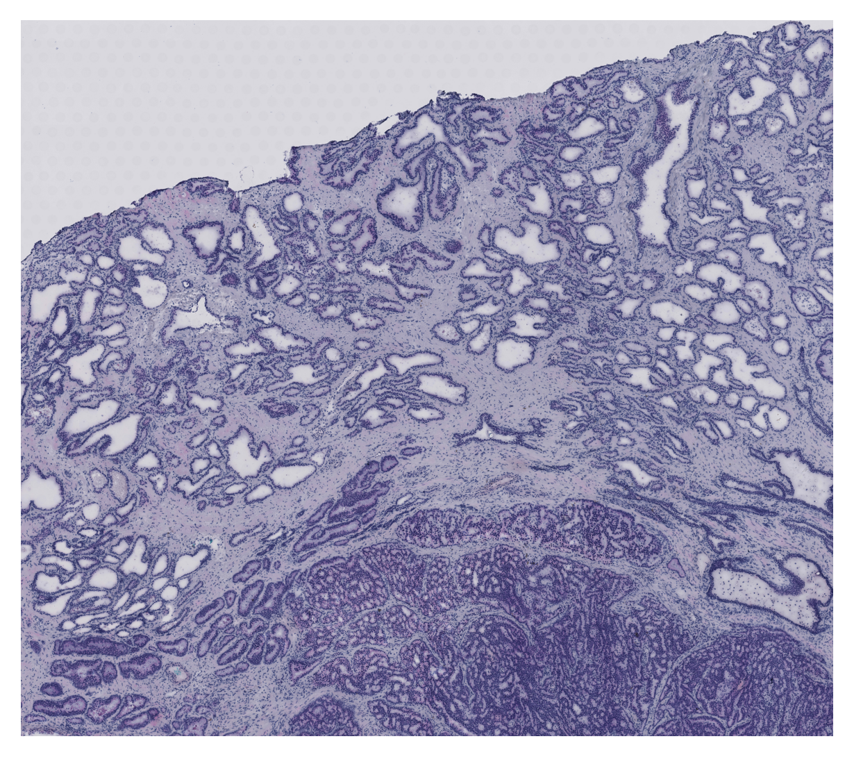
Visualize Region of Interest

Load and display the whole slide image, focusing on the selected region of interest defined by the bounding box. This visualization helps verify that the correct tissue region is being analyzed and provides spatial context for the subsequent analysis.

img_path = "../data/morph_psdtime/prostate_cancer_sample.tif"

max_side = 4000
slide = openslide.OpenSlide(img_path)
full_w, full_h = slide.dimensions

scale = max_side / max(full_w, full_h)
thumb_size = (int(full_w * scale), int(full_h * scale))

img = np.array(slide.get_thumbnail(thumb_size))  # uint8 RGB

# Convert bbox
x1, x2, y1, y2 = bbox
tx1, ty1 = int(x1 * scale), int(y1 * scale)
tx2, ty2 = int(x2 * scale), int(y2 * scale)

# Crop thumbnail
crop = img[ty1:ty2, tx1:tx2]

# Plot
plt.figure(figsize=(5, 5), dpi=150)
plt.imshow(crop)
plt.axis('off')
plt.show()

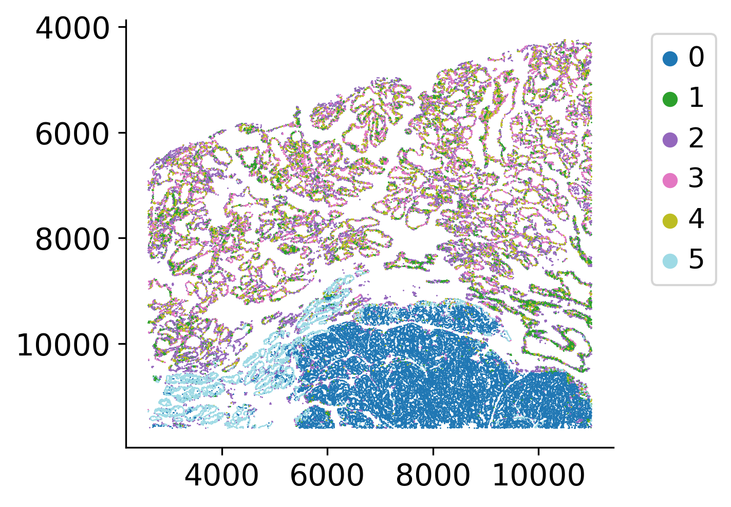
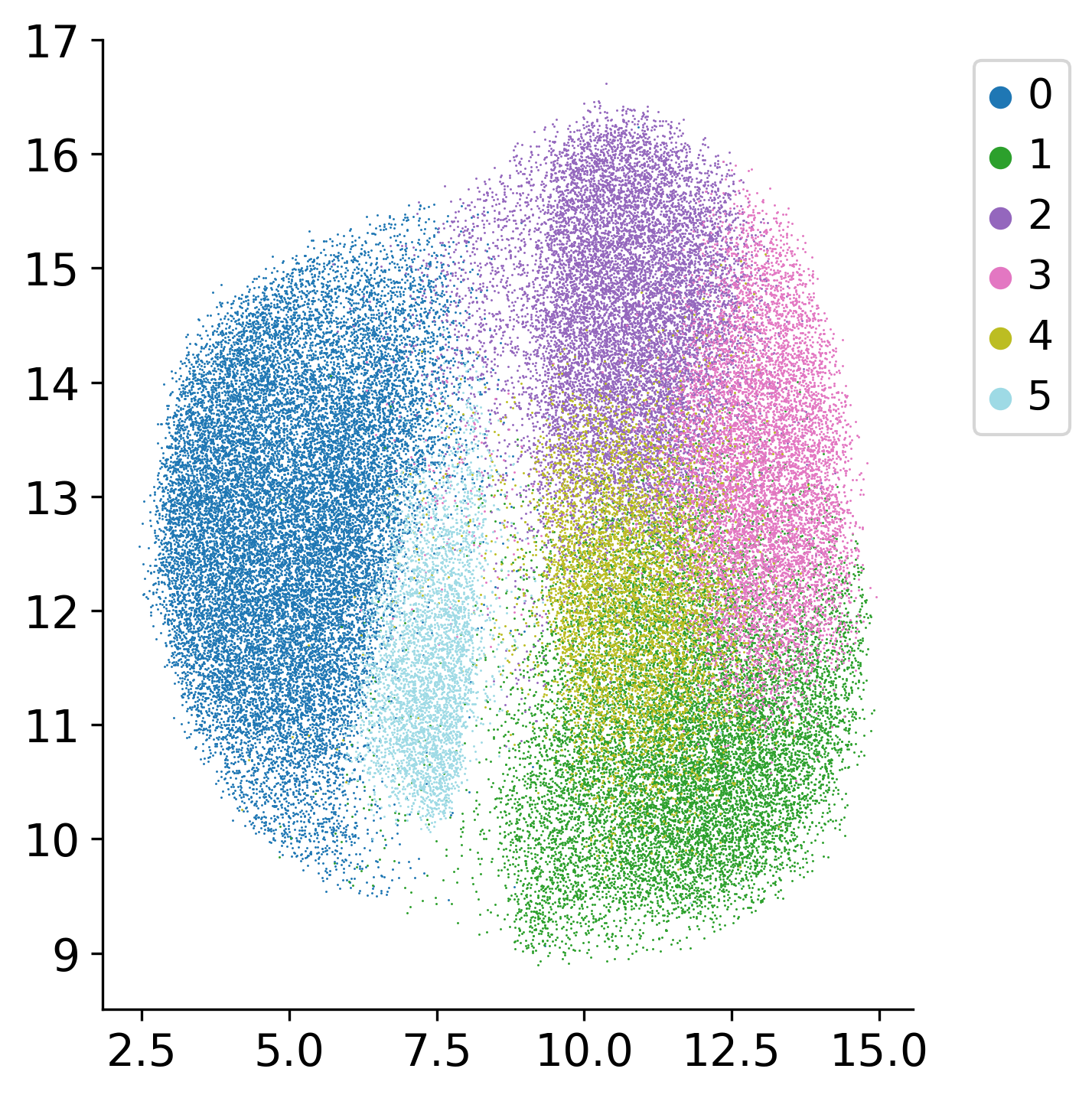
Prepare Data and Perform Clustering

Create an AnnData object from the embeddings and compute neighborhood graphs, perform Louvain clustering, and apply dimensionality reduction (UMAP). These analyses help identify distinct cell populations and capture the underlying structure of the cell state manifold, which is essential for pseudotime inference.

ad = sc.AnnData(embs.numpy())
ad.obsm['spatial'] = locs.numpy()

ad.obs['imagerow'] = ad.obsm['spatial'][:, 1]
ad.obs['imagecol'] = ad.obsm['spatial'][:, 0]

sc.pp.neighbors(ad, n_neighbors=100)

sc.tl.louvain(ad, random_state=0, resolution=1)

sc.tl.umap(ad)

loki2.plot.scatter_plot(
    ad.obsm['spatial'], 
    ad.obs['louvain'],
    s=0.5, invert_y=True, lw=0, ec=None, palette='tab20', equal_aspect=True)

loki2.plot.scatter_plot(
    ad.obsm['X_umap'][:, :2], 
    ad.obs['louvain'],
    s=0.5, invert_y=False, lw=0, ec=None, palette='tab20', equal_aspect=False)

Select Starting Cell for Pseudotime

Plot the UMAP (hover) for easier selection of an early cell. The algorithm will find a start cell near the selected cell. This interactive visualization helps identify the starting point for pseudotime inference, which represents an early developmental or progression state.

df = pd.DataFrame({
    "x": ad.obsm['X_umap'][:, 0],
    "y": ad.obsm['X_umap'][:, 1],
    "cluster": ad.obs['louvain'],
    "sx": ad.obsm['spatial'][:, 0],
    "sy": ad.obsm['spatial'][:, 1],
    "cell_id": ad.obs_names,
})

fig = px.scatter(
    df,
    x="x", y="y",
    color="cluster",
    color_discrete_sequence=px.colors.qualitative.T10,
    hover_data={
        "cluster": ":d",
        "x": ":.2f",
        "y": ":.2f",
        "sx": ":.1f",
        "sy": ":.1f",
        "cell_id": ":6d"
    },
)

fig.update_traces(marker=dict(size=3), selector=dict(mode="markers"))

legend_marker_size = 10
legend_traces = []
for trace in fig.data:
    trace.legendgroup = trace.name
    trace.showlegend = False
    legend_traces.append(
        go.Scatter(
            x=[None],
            y=[None],
            mode="markers",
            marker=dict(
                color=trace.marker.color,
                symbol=trace.marker.symbol or "circle",
                size=legend_marker_size,
            ),
            name=trace.name,
            legendgroup=trace.legendgroup,
            hoverinfo="skip",
        )
    )

fig.add_traces(legend_traces)
fig.update_layout(
    xaxis_title="UMAP-1",
    yaxis_title="UMAP-2",
    dragmode="pan"
)

fig.update_layout(width=600, height=600)
fig.show()

sc.pp.neighbors(ad, use_rep='X_umap')

Infer Pseudotime

Apply Palantir algorithm to infer pseudotime from the morphological embeddings. The algorithm uses the starting cell to define the beginning of the trajectory and computes pseudotime values for all cells based on their positions in the embedding space.

start_cell = '32100'
loki2.psdtime.infer_pseudotime_palantir(ad, start_cell, output_dir, f'PRAD-{start_cell}', n_components=15, knn=100, num_waypoints=1200)

Kept components: 12 of 12
Sampling and flocking waypoints...
Time for determining waypoints: 0.07108865181605022 minutes
Determining pseudotime...
Shortest path distances using 100-nearest neighbor graph...
Time for shortest paths: 7.433553902308146 minutes
Iteratively refining the pseudotime...
Correlation at iteration 1: 0.9999
Entropy and branch probabilities...
Markov chain construction...
Identification of terminal states...
Computing fundamental matrix and absorption probabilities...
Project results to all cells...

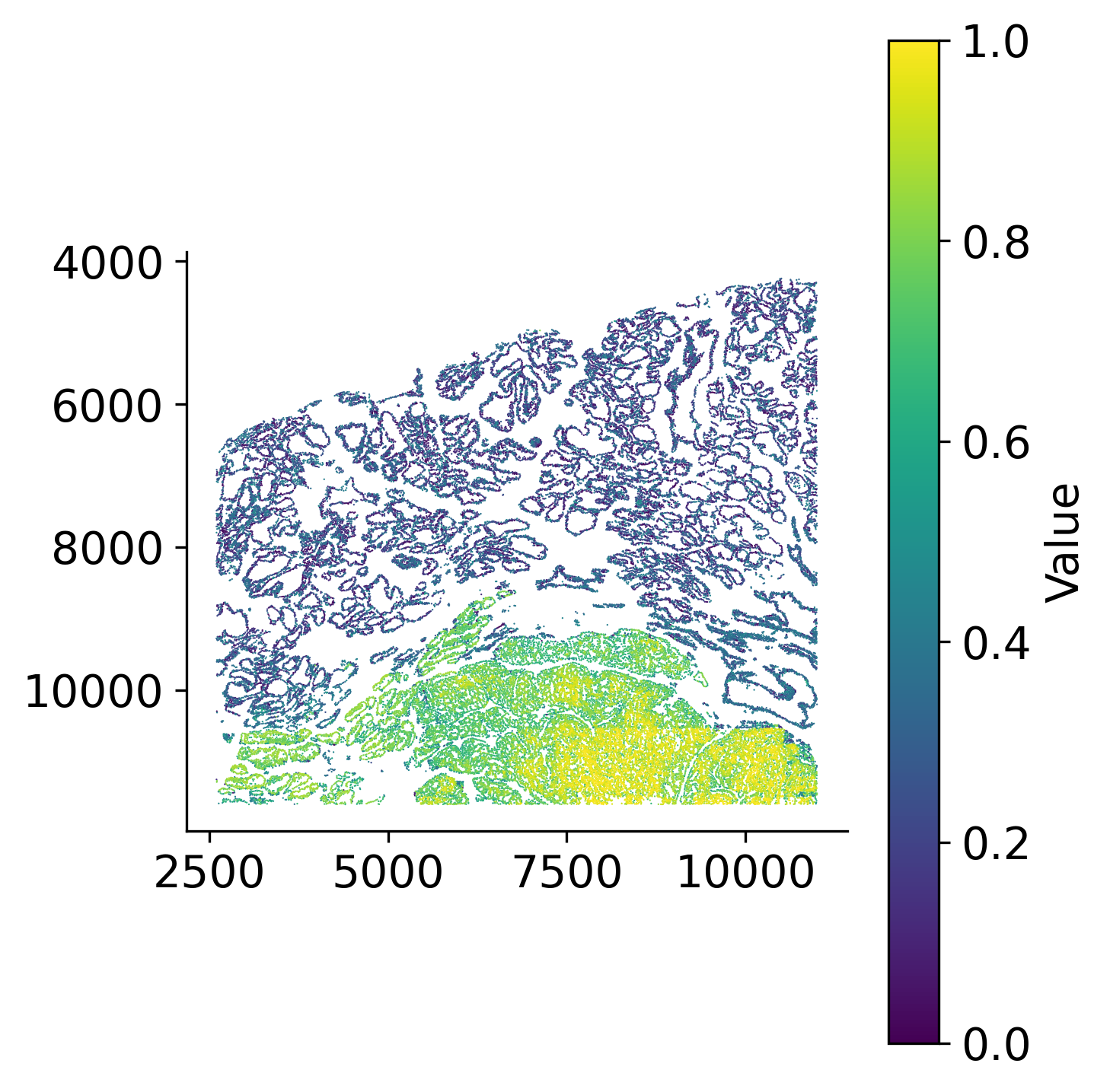
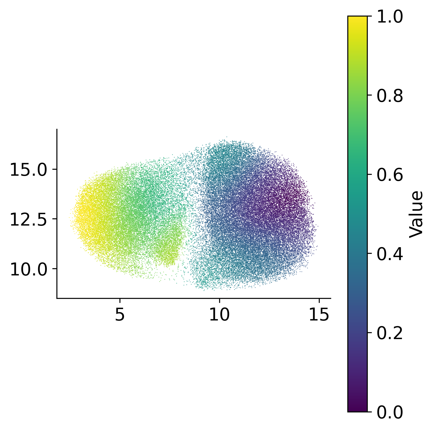
Visualize Pseudotime

Visualize the inferred pseudotime values on both spatial coordinates and UMAP embedding space. The spatial visualization shows how pseudotime progresses across the tissue, revealing regions at different stages of development or progression. The UMAP visualization shows pseudotime progression in the reduced embedding space, highlighting the trajectory structure.

loki2.plot.scatter_plot(
    ad.obsm['spatial'], 
    ad.obs['palantir_pseudotime'], 
    s=0.3, invert_y=True, lw=0, ec=None, palette='viridis',
    # save_dpi=200,
    # save_path=f"{output_dir}/pseudotime_on_spatial.jpg"
    )

loki2.plot.scatter_plot(
    ad.obsm['X_umap'][:, :2], 
    ad.obs['palantir_pseudotime'],
    s=0.3, invert_y=False, lw=0, ec=None, palette='viridis',
    # save_dpi=200,
    # save_path=f"{output_dir}/pseudotime_on_umap.jpg"
    )

Plot Trajectory

Visualize developmental trajectories and terminal states identified by Palantir. The trajectory plots show the progression paths through the cell state space, with arrows indicating the direction of progression. Terminal states represent distinct endpoints in the developmental process, and the visualization helps understand the branching structure of cellular differentiation.

masks = palantir.presults.select_branch_cells(ad, q=.01, eps=.01)

term_states = ad.obsm['palantir_fate_probabilities'].columns

for term in term_states:
    palantir.plot.plot_trajectory(
        ad, 
        term,    
        n_arrows=5, 
        cell_color="palantir_pseudotime", 
        smoothness=1, 
        scanpy_kwargs={'cmap':'viridis'},
        )

    plt.tight_layout()
    plt.gca().invert_yaxis()
    plt.gca().invert_xaxis()
    plt.show()
    # plt.savefig(f'{output_dir}/trajectory{term}_on_umap_colored_by_pseudotime.jpg', dpi=1000)
    plt.close()

[2025-12-04 12:01:27,600] [INFO    ] Using sparse Gaussian Process since n_landmarks (50) < n_samples (66,249) and rank = 1.0.
[2025-12-04 12:01:27,602] [INFO    ] Using covariance function Matern52(ls=0.7344358444213868).
[2025-12-04 12:01:27,641] [INFO    ] Computing 50 landmarks with k-means clustering (random_state=42).
[2025-12-04 12:01:31,490] [INFO    ] Sigma interpreted as element-wise standard deviation.