Case study 1: Gastrulation erythroid maturation
This tutorial shows how cellDancer analyzes RNA velocity. The process includes (1) estimating RNA velocity, (2) deriving cell fates on embedding space, and (3) estimating pseudotime.
This tutorial also demonstrates cellDancer’s ability to resolve the difficulty of predicting the velocity of genes with transcriptional boost mentioned by Barile et al.
Below is the case study for gastrulation erythroid maturation. We select 12,329 cells with 2,000 genes from haemato-endothelial progenitors, blood progenitors 1/2, and erythroid 1/2/3. The embryonic days are selected from E7.0, E7.25, E7.5, E7.75, E8.0, E8.25, and E8.5.
Import packages
To run the notebook locally, Installation could be referred to install the environment and dependencies.
[1]:
import os
import sys
import glob
import pandas as pd
import math
import matplotlib.pyplot as plt
import celldancer as cd
import celldancer.cdplt as cdplt
from celldancer.cdplt import colormap
Load data
The input data for cellDancer contains the abundances of unspliced RNA and spliced RNA. For the detail of obtaining the dataset and pre-processing steps, Data Preparation could be referred to. We follow the standard data preparation procedures in scVelo with default parameters except that we use 100 nearest neighbors for first-moment calculation.
The data of gastrulation erythroid maturation could be downloaded and unzipped from GastrulationErythroid_cell_type_u_s.csv.zip. It could be loaded by pd.read_csv('your_path/GastrulationErythroid_cell_type_u_s.csv'). To load your own data, the dataframe should contain columns ‘gene_name’, ‘unsplice’, ‘splice’ ,‘cellID’ ,‘clusters’ ,‘embedding1’ , and ‘embedding2.’ For a detailed description of the data
structure, Preprocessing could be referred to.
[2]:
cell_type_u_s_path='your_path/GastrulationErythroid_cell_type_u_s.csv'
cell_type_u_s=pd.read_csv(cell_type_u_s_path)
cell_type_u_s
[2]:
| gene_name | unsplice | splice | cellID | clusters | embedding1 | embedding2 | |
|---|---|---|---|---|---|---|---|
| 0 | Sox17 | 0.000000 | 0.043971 | cell_363 | Blood progenitors 2 | 3.460521 | 15.574629 |
| 1 | Sox17 | 0.000000 | 0.000000 | cell_382 | Blood progenitors 2 | 2.490433 | 14.971734 |
| 2 | Sox17 | 0.000000 | 0.018161 | cell_385 | Blood progenitors 2 | 2.351203 | 15.267069 |
| 3 | Sox17 | 0.000000 | 0.000000 | cell_393 | Blood progenitors 2 | 5.899098 | 14.388825 |
| 4 | Sox17 | 0.000000 | 0.000000 | cell_398 | Blood progenitors 2 | 4.823139 | 15.374831 |
| ... | ... | ... | ... | ... | ... | ... | ... |
| 24657995 | Gm47283 | 0.214961 | 1.145533 | cell_139318 | Erythroid3 | 8.032358 | 7.603037 |
| 24657996 | Gm47283 | 0.300111 | 1.072944 | cell_139321 | Erythroid3 | 10.352904 | 6.446736 |
| 24657997 | Gm47283 | 0.292607 | 1.199875 | cell_139326 | Erythroid3 | 9.464873 | 7.261099 |
| 24657998 | Gm47283 | 0.266031 | 1.114659 | cell_139327 | Erythroid3 | 9.990495 | 7.243880 |
| 24657999 | Gm47283 | 0.164675 | 1.111358 | cell_139330 | Erythroid3 | 8.260699 | 7.935455 |
24658000 rows × 7 columns
Estimate RNA velocity for sample genes
Here, 15 genes in gene_list are estimated as an example. The predicted unspliced and spliced reads, alpha, beta, and gamma are added to the dataframe.
[3]:
gene_list=['Smarca2', 'Rbms2', 'Myo1b', 'Hba-x', 'Yipf5', 'Skap1', 'Smim1', 'Nfkb1', 'Sulf2', 'Blvrb', 'Hbb-y', 'Coro2b', 'Yipf5', 'Phc2', 'Mllt3']

loss_df, cellDancer_df=cd.velocity(cell_type_u_s,\
                                   gene_list=gene_list,\
                                   permutation_ratio=0.125,\
                                   n_jobs=8)
cellDancer_df
Using /Users/shengyuli/Library/CloudStorage/OneDrive-HoustonMethodist/work/Velocity/bin/cellDancer_polish/analysis/CaseStudyNotebook/cellDancer_velocity_2022-10-20 10-11-23 as the output path.
Arranging genes for parallel job.
14  genes were arranged to  2  portions.
Velocity Estimation:   0%|          | 0/2 [00:00<?, ?it/s]
Velocity Estimation:  50%|█████     | 1/2 [00:20<00:20, 20.31s/it]
Velocity Estimation: 100%|██████████| 2/2 [00:29<00:00, 13.99s/it]
[3]:
| cellIndex | gene_name | unsplice | splice | unsplice_predict | splice_predict | alpha | beta | gamma | loss | cellID | clusters | embedding1 | embedding2 | |
|---|---|---|---|---|---|---|---|---|---|---|---|---|---|---|
| 0 | 0 | Mllt3 | 0.087552 | 0.061677 | 0.131864 | 0.347319 | 0.264903 | 0.304851 | 0.335579 | 0.111875 | cell_363 | Blood progenitors 2 | 3.460521 | 15.574629 |
| 1 | 1 | Mllt3 | 0.042049 | 0.056451 | 0.096471 | 0.192440 | 0.253070 | 0.303873 | 0.335266 | 0.111875 | cell_382 | Blood progenitors 2 | 2.490433 | 14.971734 |
| 2 | 2 | Mllt3 | 0.046162 | 0.073611 | 0.099587 | 0.222645 | 0.253818 | 0.304017 | 0.335363 | 0.111875 | cell_385 | Blood progenitors 2 | 2.351203 | 15.267069 |
| 3 | 3 | Mllt3 | 0.119952 | 0.142994 | 0.156111 | 0.534318 | 0.270146 | 0.306117 | 0.336443 | 0.111875 | cell_393 | Blood progenitors 2 | 5.899098 | 14.388825 |
| 4 | 4 | Mllt3 | 0.027221 | 0.136220 | 0.083502 | 0.221573 | 0.243896 | 0.304314 | 0.336083 | 0.111875 | cell_398 | Blood progenitors 2 | 4.823139 | 15.374831 |
| ... | ... | ... | ... | ... | ... | ... | ... | ... | ... | ... | ... | ... | ... | ... |
| 172601 | 12324 | Yipf5 | 0.098889 | 0.443361 | 0.101194 | 0.466415 | 0.080456 | 0.198707 | 0.447713 | 0.060657 | cell_139318 | Erythroid3 | 8.032358 | 7.603037 |
| 172602 | 12325 | Yipf5 | 0.092605 | 0.521375 | 0.094589 | 0.530523 | 0.074335 | 0.197698 | 0.450130 | 0.060657 | cell_139321 | Erythroid3 | 10.352904 | 6.446736 |
| 172603 | 12326 | Yipf5 | 0.108367 | 0.443695 | 0.109323 | 0.473431 | 0.081982 | 0.198220 | 0.447828 | 0.060657 | cell_139326 | Erythroid3 | 9.464873 | 7.261099 |
| 172604 | 12327 | Yipf5 | 0.067904 | 0.431785 | 0.074884 | 0.433994 | 0.076296 | 0.200459 | 0.447011 | 0.060657 | cell_139327 | Erythroid3 | 9.990495 | 7.243880 |
| 172605 | 12328 | Yipf5 | 0.077812 | 0.388213 | 0.084044 | 0.402742 | 0.080739 | 0.200674 | 0.445712 | 0.060657 | cell_139330 | Erythroid3 | 8.260699 | 7.935455 |
172606 rows × 14 columns
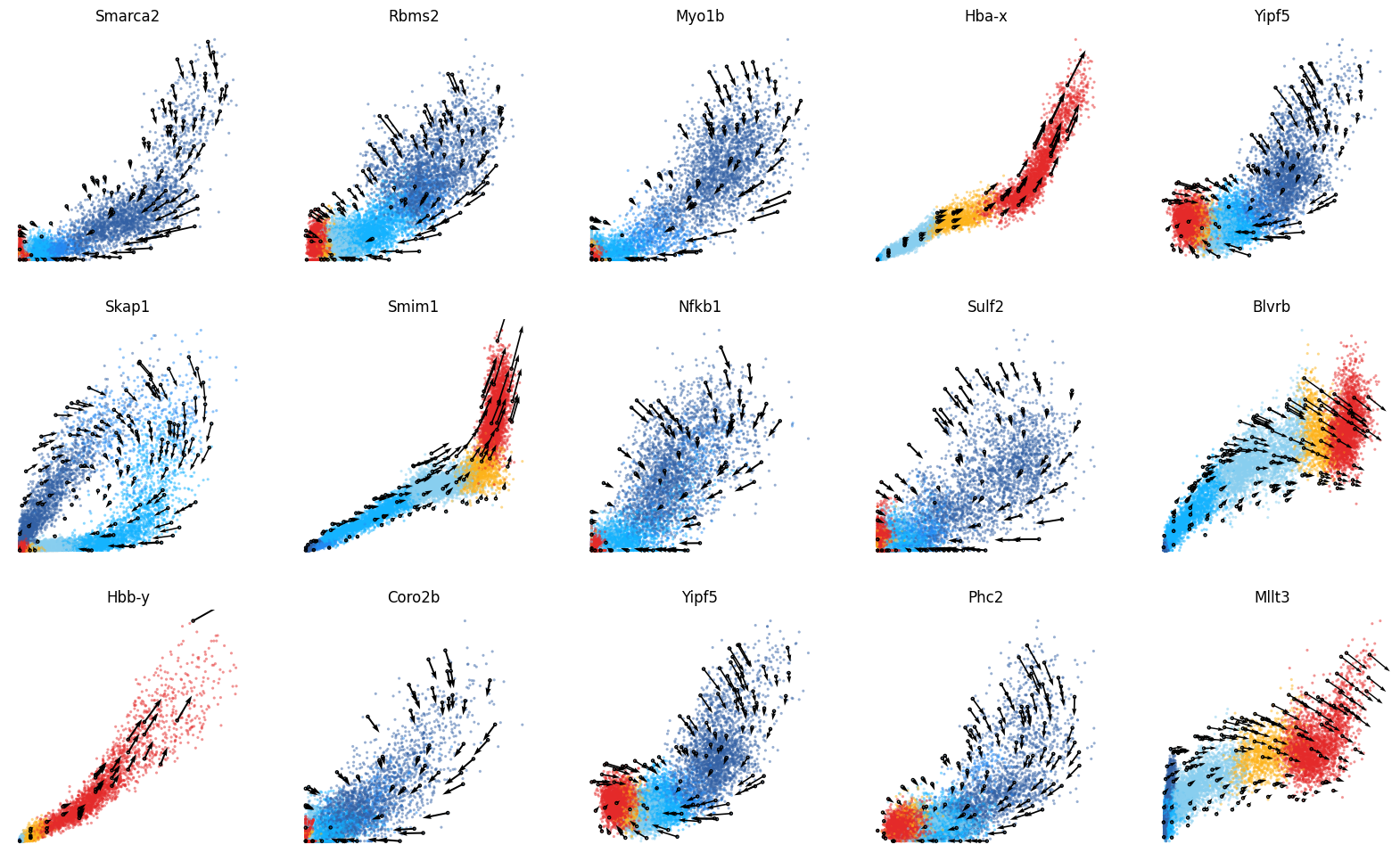
Visualize the phase portraits
We visualize the phase portrait of each gene with cdplt.scatter_gene().
From the figures below, the prediction of those genes that have transcriptional boost (Hba-x, Smim1, and Hbb-y) are consistent with the progression of gastrulation erythroid maturation of (1) haemato-endothelial progenitors, (2) blood progenitors 1/2, and (3) erythroid. This reflects the ability of cellDancer to resolve the RNA velocity for the genes in the transcriptional boost scenario.
[4]:
ncols=5
height=math.ceil(len(gene_list)/5)*4
fig = plt.figure(figsize=(20,height))

for i in range(len(gene_list)):
    ax = fig.add_subplot(math.ceil(len(gene_list)/ncols), ncols, i+1)
    cdplt.scatter_gene(
        ax=ax,
        x='splice',
        y='unsplice',
        cellDancer_df=cellDancer_df,
        custom_xlim=None,
        custom_ylim=None,
        colors=colormap.colormap_erythroid,
        alpha=0.5,
        s = 5,
        velocity=True,
        gene=gene_list[i])

    ax.set_title(gene_list[i])
    ax.axis('off')

plt.show()
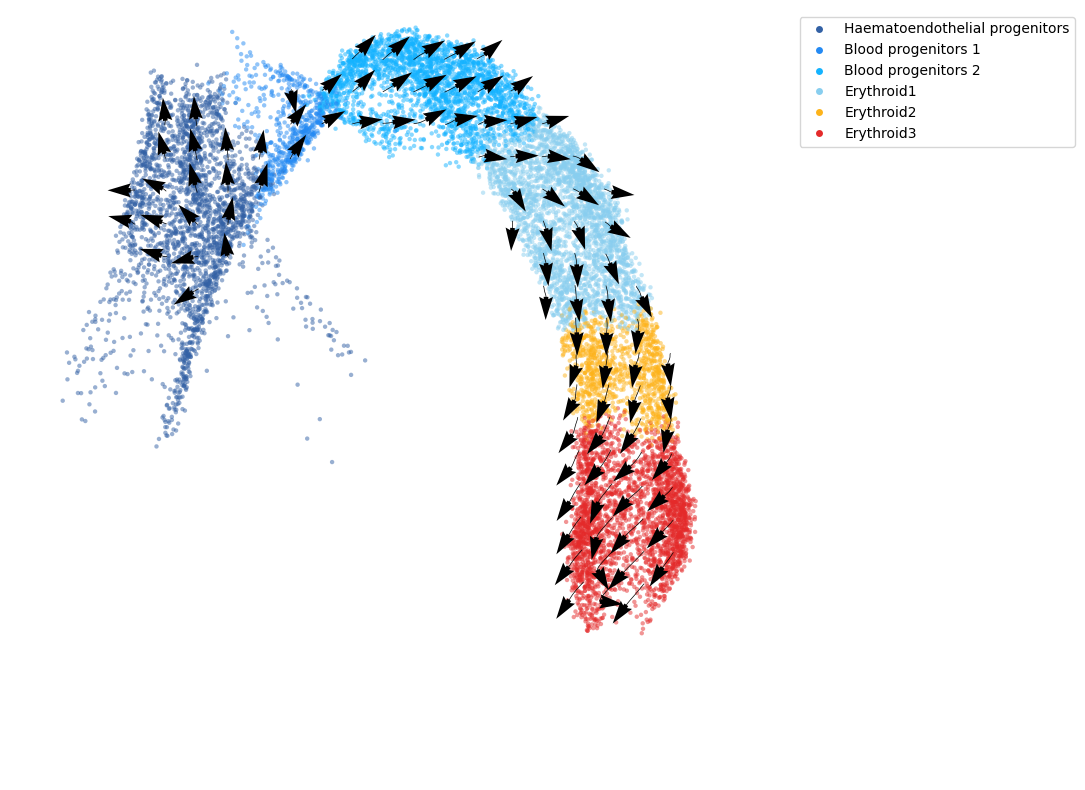
Project the RNA velocity onto the embedding space
To project the prediction of RNA velocity onto the embedding space and to estimate pseudotime using all 2,000 genes, predicted result can be downloaded from GastrulationErythroid_cellDancer_estimation.csv.zip
[5]:
# load the prediction result of all genes
cellDancer_df_path = 'your_path/GastrulationErythroid_cellDancer_estimation.csv'
cellDancer_df = pd.read_csv(cellDancer_df_path)
We calculate the projection of RNA velocity on the embedding with cd.compute_cell_velocity(). The projected direction on embedding space, i.e. columns ‘velocity1’ and ‘velocity2’ are added to the original dataframe. We use cdplt.scatter_cell() to display the predicted direction on embedding space.
[6]:
# compute cell velocity
cellDancer_df=cd.compute_cell_velocity(cellDancer_df=cellDancer_df, projection_neighbor_choice='gene', expression_scale='power10', projection_neighbor_size=10, speed_up=(100,100))

# plot cell velocity
fig, ax = plt.subplots(figsize=(10,10))
cdplt.scatter_cell(ax,
                   cellDancer_df,
                   colors=colormap.colormap_erythroid,
                   alpha=0.5,
                   s=10,
                   velocity=True,
                   legend='on',
                   min_mass=15,
                   arrow_grid=(20,20),
                   custom_xlim=[-6,13],
                   custom_ylim=[2,16], )
ax.axis('off')
plt.show()
[7]:
cellDancer_df
[7]:
| cellIndex | gene_name | unsplice | splice | unsplice_predict | splice_predict | alpha | beta | gamma | loss | cellID | clusters | embedding1 | embedding2 | index | velocity1 | velocity2 | |
|---|---|---|---|---|---|---|---|---|---|---|---|---|---|---|---|---|---|
| 0 | 0 | Ift81 | 0.010658 | 0.026321 | 0.009261 | 0.029549 | 0.023595 | 0.042598 | 0.073999 | 0.039626 | cell_363 | Blood progenitors 2 | 3.460521 | 15.574629 | 0 | NaN | NaN |
| 1 | 1 | Ift81 | 0.000000 | 0.044266 | 0.000946 | 0.037888 | 0.020649 | 0.042942 | 0.074502 | 0.039626 | cell_382 | Blood progenitors 2 | 2.490433 | 14.971734 | 1 | NaN | NaN |
| 2 | 2 | Ift81 | 0.000000 | 0.064559 | 0.000885 | 0.055191 | 0.019326 | 0.042876 | 0.075031 | 0.039626 | cell_385 | Blood progenitors 2 | 2.351203 | 15.267069 | 2 | NaN | NaN |
| 3 | 3 | Ift81 | 0.000000 | 0.020756 | 0.001014 | 0.017791 | 0.022149 | 0.043030 | 0.073879 | 0.039626 | cell_393 | Blood progenitors 2 | 5.899098 | 14.388825 | 3 | NaN | NaN |
| 4 | 4 | Ift81 | 0.000000 | 0.013184 | 0.001037 | 0.011305 | 0.022633 | 0.043055 | 0.073676 | 0.039626 | cell_398 | Blood progenitors 2 | 4.823139 | 15.374831 | 4 | NaN | NaN |
| ... | ... | ... | ... | ... | ... | ... | ... | ... | ... | ... | ... | ... | ... | ... | ... | ... | ... |
| 24657995 | 12324 | Mcrip1 | 0.000000 | 1.128435 | 0.000157 | 1.125867 | 0.005920 | 0.038023 | 0.013131 | 0.051755 | cell_139318 | Erythroid3 | 8.032358 | 7.603037 | 12324 | NaN | NaN |
| 24657996 | 12325 | Mcrip1 | 0.024356 | 0.970672 | 0.016090 | 1.428982 | 0.008338 | 0.037053 | 0.013950 | 0.051755 | cell_139321 | Erythroid3 | 10.352904 | 6.446736 | 12325 | NaN | NaN |
| 24657997 | 12326 | Mcrip1 | 0.000000 | 0.899107 | 0.000175 | 0.897000 | 0.006575 | 0.037644 | 0.013522 | 0.051755 | cell_139326 | Erythroid3 | 9.464873 | 7.261099 | 12326 | NaN | NaN |
| 24657998 | 12327 | Mcrip1 | 0.017375 | 1.398107 | 0.011387 | 1.729827 | 0.006885 | 0.037765 | 0.013271 | 0.051755 | cell_139327 | Erythroid3 | 9.990495 | 7.243880 | 12327 | NaN | NaN |
| 24657999 | 12328 | Mcrip1 | 0.005194 | 0.988933 | 0.003540 | 1.086199 | 0.006822 | 0.037569 | 0.013596 | 0.051755 | cell_139330 | Erythroid3 | 8.260699 | 7.935455 | 12328 | NaN | NaN |
24658000 rows × 17 columns
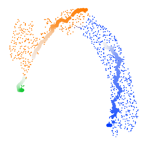
Estimate pseudotime
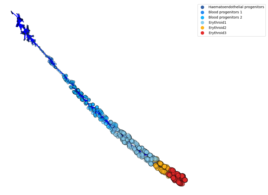
Based on the projection of RNA velocity on embedding space, we estimate the pseudotime with cd.pseudo_time().
The long trajectories used for pseudotime dertermination are (optionally) shown. In this case, the three long trajectories are colored from light to dark according to their own unadjusted pseudotime. The cells are colored according to the long trajectories that are used for determination of the pseudotime of the cells.
[8]:
import random
# set parameters
dt = 0.05
t_total = {dt:int(10/dt)}
n_repeats = 10

# estimate pseudotime
cellDancer_df = cd.pseudo_time(cellDancer_df=cellDancer_df,
                               grid=(30,30),
                               dt=dt,
                               t_total=t_total[dt],
                               n_repeats=n_repeats,
                               speed_up=(100,100),
                               n_paths = 3,
                               plot_long_trajs=True,
                               psrng_seeds_diffusion=[i for i in range(n_repeats)],
                               n_jobs=8)
Pseudo random number generator seeds are set to: [0, 1, 2, 3, 4, 5, 6, 7, 8, 9]
Generating Trajectories: 100%|████████████| 9510/9510 [00:02<00:00, 3175.15it/s]
There are 3 clusters.
[0 1 2]
--- 257.67111110687256 seconds ---
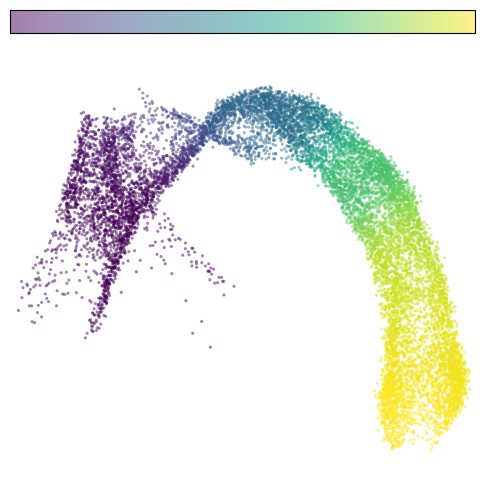
[9]:
# plot pseudotime
fig, ax = plt.subplots(figsize=(6,6))
im=cdplt.scatter_cell(ax,cellDancer_df, colors='pseudotime', alpha=0.5, velocity=False, custom_xlim=(-5,11), custom_ylim=(4,18))
ax.axis('off')
plt.show()
The connection network below is another method to display pseudotime (cdplt.PTO_Graph). The edge lengths indicate the time difference between nodes (the closer in pseudotime, the shorter the edge length). The sizes of the nodes are proportional to the pseudotime.
[10]:
fig, ax= plt.subplots(figsize=(10,10))

cdplt.PTO_Graph(ax,
                cellDancer_df,
                node_layout='forcedirected',
                PRNG_SEED=10,
                use_edge_bundling=True,
                node_colors=colormap.colormap_erythroid,
                edge_length=3,
                node_sizes='pseudotime',
                colorbar='on',
                legend='on')
[10]:
<AxesSubplot:>
Display the abundance of spliced RNA along pseudotime
We visualize the spliced RNA abundance of genes along pseudotime with cdplt.scatter_gene().
[11]:
ncols=5
height=math.ceil(len(gene_list)/ncols)*4
fig = plt.figure(figsize=(20,height))

for i in range(len(gene_list)):
    ax = fig.add_subplot(math.ceil(len(gene_list)/ncols), ncols, i+1)
    cdplt.scatter_gene(
        ax=ax,
        x='pseudotime',
        y='splice',
        cellDancer_df=cellDancer_df,
        custom_xlim=None,
        custom_ylim=None,
        colors=colormap.colormap_erythroid,
        alpha=0.5,
        s = 5,
        velocity=False,
        gene=gene_list[i])

    ax.set_title(gene_list[i])
    ax.axis('off')
