Case Study 2: Mouse hippocampus development

This tutorial shows how cellDancer analyzes RNA velocity. The process includes (1) estimating RNA velocity, (2) deriving cell fates on embedding space, (3) estimating pseudotime, and (4) displaying predicted kinetics rates (transcription, splicing, and degradation rates), spliced mRNA abundance, and unspliced mRNA abundance on embedding space.

Below is the case study for the mouse hippocampal dentate gyrus neurogenesis. We follow the preprocessing methods of La Manno et al. to filter genes and cells. 18,140 cells with 2,159 genes were selected.

Import packages

To run the notebook locally, Installation could be referred to install the environment and dependencies.

# import packages
import os
import sys
import glob
import pandas as pd
import math
import matplotlib.pyplot as plt
import celldancer as cd
import celldancer.cdplt as cdplt
from celldancer.cdplt import colormap

Load data

The input data for cellDancer contains the preprocessed abundances of unspliced RNA and spliced RNA. The data of mouse hippocampal dentate gyrus neurogenesis can be ownloaded from DentateGyrus_cell_type_u_s.csv.zip. To load your own data, the dataframe should contain columns ‘gene_name’, ‘unsplice’, ‘splice’ ,‘cellID’ ,‘clusters’ ,‘embedding1’, and ‘embedding2.’ For a detailed description about the preprocessing and the data structure, refer to Data Preparation.

cell_type_u_s_path="your_path/DentateGyrus_cell_type_u_s.csv"
cell_type_u_s=pd.read_csv(cell_type_u_s_path)
cell_type_u_s

	gene_name	unsplice	splice	cellID	clusters	embedding1	embedding2
0	Rgs20	0.069478	0.021971	10X83_2:AAACGGGGTCTCTTTAx	ImmGranule2	18.931086	-1.862429
1	Rgs20	0.085834	0.016256	10X83_2:AACCATGGTTCAACCAx	ImmGranule2	18.419891	-1.282895
2	Rgs20	0.068644	0.047774	10X83_2:AACACGTTCTGAAAGAx	CA2-3-4	2.369887	16.868419
3	Rgs20	0.045387	0.018101	10X83_2:AAAGATGCATTGAGCTx	CA	-5.351040	10.676485
4	Rgs20	0.040457	0.012846	10X83_2:AACCATGTCTACTTACx	CA1-Sub	-6.189126	11.754900
...	...	...	...	...	...	...	...
39164255	Gpm6b	0.876650	1.276089	10X84_3:TTTCCTCCACCATCCTx	ImmGranule1	10.812611	-2.487668
39164256	Gpm6b	2.024897	5.152006	10X84_3:TTTGTCACATGAAGTAx	CA2-3-4	8.246204	23.482788
39164257	Gpm6b	1.848051	1.491445	10X84_3:TTTCCTCCACGGTAAGx	nIPC	-3.441272	-4.917364
39164258	Gpm6b	0.696361	1.189091	10X84_3:TTTGTCAAGCGTCAAGx	ImmGranule2	16.394199	-6.143549
39164259	Gpm6b	0.739348	1.239052	10X84_3:TTTCCTCGTGAAAGAGx	ImmGranule2	17.490857	-4.130190

39164260 rows × 7 columns

Estimate RNA velocity for sample genes

We use cd.velocity() to estimate the velocity. Here, 30 genes in gene_list are estimated as an example. The predicted unspliced and spliced reads, alpha, beta, and gamma are added to the dataframe.

gene_list=['Psd3', 'Dcx', 'Syt11', 'Ntrk2', 'Gnao1', 'Gria1', 'Dctn3', 'Map1b', 'Camk2a', 'Gpm6b', 'Sez6l', 'Evl', 'Astn1', 'Ank2', 'Klf7', 'Tbc1d16', 'Atp1a3', 'Stxbp6', 'Scn2a1', 'Lhx9', 'Slc4a4', 'Ppfia2', 'Kcnip1', 'Ptpro', 'Diaph3', 'Slc1a3', 'Cadm1', 'Mef2c', 'Sptbn1', 'Ncald']

loss_df, cellDancer_df=cd.velocity(cell_type_u_s,
                                   gene_list=gene_list,
                                   permutation_ratio=0.1,
                                   norm_u_s=False,
                                   norm_cell_distribution=False,
                                   n_jobs=8)
cellDancer_df

Using /Users/shengyuli/Library/CloudStorage/OneDrive-HoustonMethodist/work/Velocity/bin/cellDancer_polish/analysis/CaseStudyNotebook/cellDancer_velocity_2022-06-27 16-37-44 as the output path.
Arranging genes for parallel job.
30  genes were arranged to  4  portions.

Velocity Estimation:   0%|          | 0/4 [00:00<?, ?it/s]
Velocity Estimation:  25%|██▌       | 1/4 [00:37<01:53, 37.68s/it]
Velocity Estimation:  50%|█████     | 2/4 [01:04<01:03, 31.53s/it]
Velocity Estimation:  75%|███████▌  | 3/4 [01:31<00:29, 29.08s/it]
Velocity Estimation: 100%|██████████| 4/4 [01:52<00:00, 26.11s/it]

	cellIndex	gene_name	unsplice	splice	unsplice_predict	splice_predict	alpha	beta	gamma	loss	cellID	clusters	embedding1	embedding2
0	0	Klf7	0.408467	1.294797	0.444935	1.475828	0.454905	0.935128	0.015373	0.077489	10X83_2:AAACGGGGTCTCTTTAx	ImmGranule2	18.931086	-1.862429
1	1	Klf7	0.379136	1.256870	0.411796	1.424216	0.419835	0.935061	0.015772	0.077489	10X83_2:AACCATGGTTCAACCAx	ImmGranule2	18.419891	-1.282895
2	2	Klf7	0.893599	3.395004	0.969404	3.832591	1.033540	0.986942	0.001990	0.077489	10X83_2:AACACGTTCTGAAAGAx	CA2-3-4	2.369887	16.868419
3	3	Klf7	0.640505	2.739187	0.669036	3.047821	0.684626	0.979797	0.003759	0.077489	10X83_2:AAAGATGCATTGAGCTx	CA	-5.351040	10.676485
4	4	Klf7	0.662303	2.433943	0.712970	2.749427	0.745024	0.971894	0.005226	0.077489	10X83_2:AACCATGTCTACTTACx	CA1-Sub	-6.189126	11.754900
...	...	...	...	...	...	...	...	...	...	...	...	...	...	...
544195	18135	Kcnip1	0.018745	0.005679	0.243844	0.008779	0.463909	0.731405	1.322285	0.079982	10X84_3:TTTCCTCCACCATCCTx	ImmGranule1	10.812611	-2.487668
544196	18136	Kcnip1	0.148039	0.093618	0.380534	0.085685	0.572677	0.727422	1.319759	0.079982	10X84_3:TTTGTCACATGAAGTAx	CA2-3-4	8.246204	23.482788
544197	18137	Kcnip1	0.080708	0.032079	0.312729	0.040230	0.522807	0.728119	1.323665	0.079982	10X84_3:TTTCCTCCACGGTAAGx	nIPC	-3.441272	-4.917364
544198	18138	Kcnip1	0.078976	0.033418	0.310343	0.040067	0.520257	0.728360	1.323348	0.079982	10X84_3:TTTGTCAAGCGTCAAGx	ImmGranule2	16.394199	-6.143549
544199	18139	Kcnip1	0.050686	0.019074	0.279029	0.024949	0.493671	0.729688	1.322998	0.079982	10X84_3:TTTCCTCGTGAAAGAGx	ImmGranule2	17.490857	-4.130190

544200 rows × 14 columns

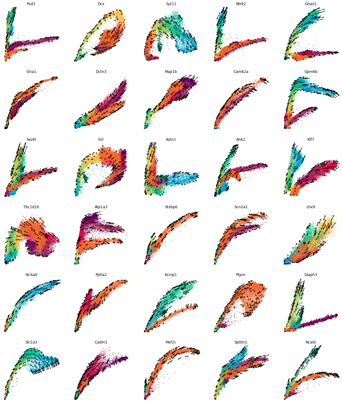
Visualize the phase portraits

We visualize the phase portrait of each gene with cdplt.scatter_gene().

ncols=5
height=math.ceil(len(gene_list)/ncols)*4
fig = plt.figure(figsize=(20,height))

for i in range(len(gene_list)):
    ax = fig.add_subplot(math.ceil(len(gene_list)/ncols), ncols, i+1)
    cdplt.scatter_gene(
        ax=ax,
        x='splice',
        y='unsplice',
        cellDancer_df=cellDancer_df,
        custom_xlim=None,
        custom_ylim=None,
        colors=colormap.colormap_neuro,
        alpha=0.5,
        s = 10,
        velocity=True,
        gene=gene_list[i])

    ax.set_title(gene_list[i])
    ax.axis('off')

plt.show()

Project the RNA velocity onto the embedding space

To project the prediction of RNA velocity to velocity onto the embedding space and to estimate pseudotime by using all genes, predicted result can be downloaded from DentateGyrus_cellDancer_estimation.csv.zip.

# load the prediction result of all genes
cellDancer_df_file = 'your_path/DentateGyrus_cellDancer_estimation.csv'
cellDancer_df=pd.read_csv(cellDancer_df_file)

We calculate the projection of RNA velocity on the embedding with cd.compute_cell_velocity(). The projected direction on embedding space, i.e. columns ‘velocity1’ and ‘velocity2’ are added to the original dataframe. We use cdplt.scatter_cell() to display the predicted direction on embedding space.

# compute cell velocity
cellDancer_df=cd.compute_cell_velocity(cellDancer_df=cellDancer_df)

# plot cell velocity
fig, ax = plt.subplots(figsize=(15,15))
im = cdplt.scatter_cell(ax,cellDancer_df,
                        colors=colormap.colormap_neuro,
                        alpha=0.3,
                        s=10,
                        velocity=True,
                        legend='on',
                        min_mass=2,
                        arrow_grid=(30,30))
ax.axis('off')
plt.show()

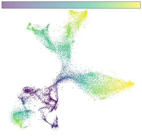
Estimate pseudotime

Based on the projection of RNA velocity on embedding space, we estimate the pseudotime with cd.pseudo_time().

%%capture

# set parameters
dt = 0.001
t_total = {dt: 10000}
n_repeats = 10

# estimate pseudotime
cellDancer_df = cd.pseudo_time(cellDancer_df=cellDancer_df,
                                          grid=(30, 30),
                                          dt=dt,
                                          t_total=t_total[dt],
                                          n_repeats=n_repeats,
                                          speed_up=(60,60),
                                          n_paths = 5,
                                          psrng_seeds_diffusion=[i for i in range(n_repeats)],
                                          n_jobs=8)

# plot pseudotime
fig, ax = plt.subplots(figsize=(10,10))
im=cdplt.scatter_cell(ax,cellDancer_df, colors='pseudotime', alpha=0.5, velocity=False)
ax.axis('off')
plt.show()

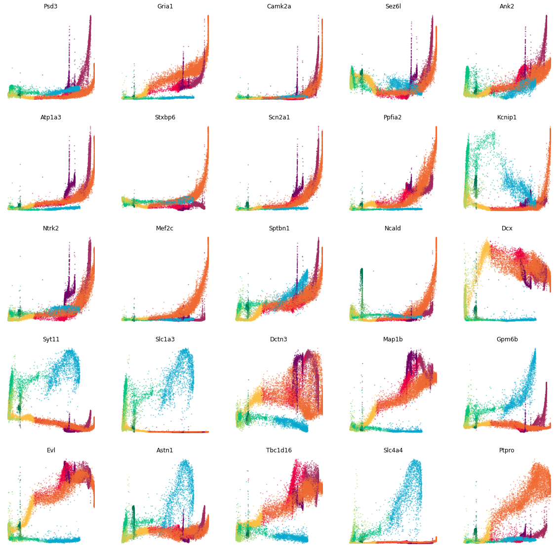
Display the abundance of spliced RNA along pseudotime

We visualize the spliced RNA abundance of some sample genes along pseudotime with cdplt.scatter_gene().

gene_list=['Psd3', 'Gria1', 'Camk2a', 'Sez6l', 'Ank2', 'Atp1a3', 'Stxbp6', 'Scn2a1', 'Ppfia2', 'Kcnip1', 'Ntrk2', 'Mef2c', 'Sptbn1', 'Ncald','Dcx', 'Syt11','Slc1a3', 'Dctn3', 'Map1b', 'Gpm6b', 'Evl', 'Astn1', 'Tbc1d16','Slc4a4', 'Ptpro']

ncols=5
height=math.ceil(len(gene_list)/ncols)*4
fig = plt.figure(figsize=(20,height))

for i in range(len(gene_list)):
    ax = fig.add_subplot(math.ceil(len(gene_list)/ncols), ncols, i+1)
    cdplt.scatter_gene(
        ax=ax,
        x='pseudotime',
        y='splice',
        cellDancer_df=cellDancer_df,
        custom_xlim=None,
        custom_ylim=None,
        colors=colormap.colormap_neuro,
        alpha=0.5,
        s = 5,
        velocity=False,
        gene=gene_list[i])

    ax.set_title(gene_list[i])
    ax.axis('off')

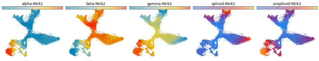
Visualize the reaction rates, the abundance of unspliced RNA, and the abundance of spliced RNA on embedding space

cellDancer provides other functions for visualization. we show the predicted kinetics rates (transcription, splicing, and degradation rates), spliced mRNA abundance, and unspliced mRNA abundance on embedding space with cdplt.scatter_cell().

gene_samples=['Ntrk2','Psd3','Dcx']

for gene in gene_samples:
    fig, ax = plt.subplots(ncols=5, figsize=(15,3))
    cdplt.scatter_cell(ax[0],cellDancer_df, colors='alpha',
                 gene=gene, velocity=False)
    cdplt.scatter_cell(ax[1],cellDancer_df, colors='beta',
                 gene=gene, velocity=False)
    cdplt.scatter_cell(ax[2],cellDancer_df, colors='gamma',
                 gene=gene, velocity=False)
    cdplt.scatter_cell(ax[3],cellDancer_df, colors='splice',
                 gene=gene, velocity=False)
    cdplt.scatter_cell(ax[4],cellDancer_df, colors='unsplice',
                 gene=gene, velocity=False)
    ax[0].axis('off')
    ax[1].axis('off')
    ax[2].axis('off')
    ax[3].axis('off')
    ax[4].axis('off')
    ax[0].set_title('alpha-'+gene)
    ax[1].set_title('beta-'+gene)
    ax[2].set_title('gamma-'+gene)
    ax[3].set_title('spliced-'+gene)
    ax[4].set_title('unspliced-'+gene)
    plt.tight_layout()
    plt.show()